Basic Usage of tmap
This guide is to help you start working with tmap.
High dimension and complex data are common in modern biological science, especially in omics studies. To successfully apply machine learning techniques in this scenario, we need to perform dimensionality reduction to have a lower dimensional representation of the data. The learned low-dimensional features can then be used for visualization or as input for regression / classification analysis.
tmap is a method which can be used to reduce high dimensional data sets into simplicial complexes with far fewer representative data points (as nodes in a TDA network), which capture topological information (” the shape of data”) at a specified resolution.
Let’s start a tmap analysis by using a simplest case, to get you familiar with the basic steps and the overall workflow.
A Simple Case
Using the classical iris dataset as a simple example. This case is use to demonstrate the general usage of tmap with simplicity in mind. The same approach can also be applied to microbiome data analysis, which will be demonstrated in this documentation.
from sklearn import datasets
import pandas as pd
iris = datasets.load_iris()
X = iris.data
X = pd.DataFrame(X,columns = iris.feature_names)
Once we have prepared input data (in pandas DataFrame or a numpy matrix), we can proceed to initiate the basic instances for TDA analysis, including Mapper, filter, cluster and Cover.
from tmap.tda import mapper, Filter
from tmap.tda.cover import Cover
from sklearn.cluster import DBSCAN
from sklearn.preprocessing import StandardScaler,MinMaxScaler
# Step1. initiate a Mapper
tm = mapper.Mapper(verbose=1)
# Step2. Projection
lens = [Filter.MDS(components=[0, 1],random_state=100)]
projected_X = tm.filter(X, lens=lens)
clusterer = DBSCAN(eps=0.75, min_samples=1)
cover = Cover(projected_data=MinMaxScaler().fit_transform(projected_X), resolution=20, overlap=0.75)
After preparing the required instances and input data, the map function of the Mapper object can be called to return a TDA graph (or TDA network). A graph is a collection of nodes (vertices) along with identified pairs of nodes (edges). For now, we use nest dictionary as a container to store all the information of a TDA graph, which will be used for TDA network visualization and statistical analysis.
graph = tm.map(data=StandardScaler().fit_transform(X), cover=cover, clusterer=clusterer)
The generated graph consists of 201 nodes and 1020 edges, which can be obtained by:
print(len(graph.nodes),len(graph.edges))

197 913
If you install the latest version of tmap==v1.2, the Graph which tmap generated has been implemented based on networkx.Graph. It could help us to save a lot of time to access the attributes of graph. If you are not familiar with networkx, you could see the documentation at networkx documentation For avoiding meet any version conflict, we force the version of networkx equal to v2.2. If there are any update, we will follow closely at the first time.
Using Different Distance Metric
After introducing the basic usage of tmap, we now delve into the details of each class. We may want to use a different distance metric instead of the default (Euclidean) distance metric. Particularly in microbiome data analysis, the weighted or unweighted UniFrac distance metric can be used.
For using custom distance metric from a precomputed distance matrix, you need to set the metric parameter as “precomputed” when initiating a filter object.
from scipy.spatial.distance import pdist,squareform
from tmap.tda.metric import Metric
lens = [Filter.MDS(components=[0, 1],metric=Metric('precomputed'))]
my_dist = squareform(pdist(X.values,metric="braycurtis"))
projected_X = tm.filter(my_dist, lens=lens)
A Filter is a general technique to project data points from the original data space onto a low dimensional space. Different filter preserves different aspect of the original dataset, such as MDS, which try to preserve distances between data points. Therefore, a filter provides a view of the data to look through. Multiple views can be joined to present the data for topological analysis. Choice of filter depends on the studied dataset and research purpose. Projection of the original dataset using a specified filter has a global effect in determining the TDA network structure.
Different filters can be generated and combined into a lens using a Python list, and within each filter, different components can be specified with a index list. There are various filters implemented in the filter module, including PCA, MDS, and t-SNE. More filters can be easily incorporated using the defined APIs.
t
TDA Network Visualization and Coloring
After constructing a TDA graph, it is very useful and insightful to visualize the network for pattern discovery. We built wrapper classes around networkx and matplotlib to facilitate TDA network visualization for different target features using a specified color mapping object.
Different with
from tmap.tda.plot import Color
y = iris.target
color = Color(target=y, dtype="categorical",target_by='sample')
graph.show(color=color, fig_size=(10, 10), node_size=15)

Depending on the type of target data, there are two types of color mappings (categorical or numerical) we can choose. If we have a binary/continuous numeric feature, we recommend using the numerical type to show a ‘node averaged’ distribution of the target feature among the network. For a binary feature, the value of a node indicates the ratio of True among all samples in the node for the feature.
For a multi-classes feature, you should use the categorical type to visualize the most-abundant category for each node. As an alternative, you can also use the One-Hot encoding method to transform a multi-classes feature into multiple binary features and then examine them individually using a numerical color map.
Network Enrichment and the SAFE score
After obtaining a TDA graph, we can explore network structures associated with the dataset and perform network based statistical analysis. One straightforward way is to use network enrichment analysis to understand how a target feature is enriched locally with a subset of nodes and groups of samples, or how the target feature vary among the whole network to have a global picture. We adopted the SAFE (Spatial Analysis of Functional Enrichment) algorithm for the calculation of a SAFE score for each node, given a specified target feature. Target feature can be a dependent variable for a supervised learning task, or can be a independent variable to identify the most distinctive attributes for a group of samples in the network.
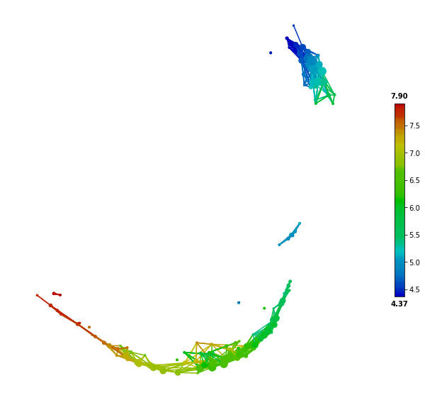
First, we plot and color the first feature (sepal length) of the iris dataset on the TDA network.
color = Color(target=X.iloc[:,0], dtype="numerical",target_by='sample')
graph.show(color=color, fig_size=(10, 10), node_size=15)
Besides the matplotlib implemented function graph.show, we also implement other function based on plotly which could display inactivated.
from tmap.tda.plot import vis_progressX, Color
color = Color(target=X.iloc[:,0], dtype="numerical")
vis_progressX(graph,simple=True,mode='file',color=Color(target=X.iloc[:,0], dtype="numerical"),filename='example1.html',auto_open=False)
From the above figure, feature coloring shows that sepal length is strongly associated with the network structure (range of the sepal length values and their color mapping are indicated by the color legend on the right-hand side). Then we can use the SAFE algorithm to transform the raw feature values to network-based statistical scores (log10-transformed p-values). SAFE_batch will return a dataframe with same columns as the inputted metadata but with different rows.
from tmap.netx.SAFE import *
safe_scores = SAFE_batch(graph, metadata=X, n_iter=1000,_mode='enrich')
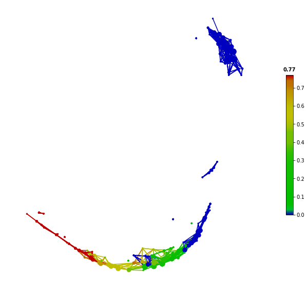
color = Color(target=safe_scores.iloc[:,0], dtype="numerical",target_by="node")
graph.show(color=color, fig_size=(10, 10), node_size=15)
from tmap.netx.SAFE import *
safe_scores = SAFE_batch(graph, metadata=X, n_iter=1000,_mode='enrich')
color = Color(target=safe_scores.iloc[:,0], dtype="numerical",target_by="node")
vis_progressX(graph,simple=True,mode='file',color=color,filename='example2.html',auto_open=False)
Instead of coloring based on original feature value, the SAFE score colors can help to reveal significantly enriched nodes in the network, which can be extracted for further analysis. Regarding the details of the SAFE algorithm and SAFE score, please see How tmap work.
SAFE Statistical Summary
In addition to the use of SAFE score for feature coloring and visualization, various network enrichment statistics can be calculated and summarized for each target feature, based on the SAFE algorithm. These statistics are useful for ranking and filtering of significant features associated with the TDA network, together with their strength of association/enrichment. The selected features are expected to explain the network structure, and therefore ‘the shape of data’.
from tmap.netx.SAFE import get_SAFE_summary
safe_summary = get_SAFE_summary(graph=graph, metadata=X, safe_scores=safe_scores,
                                n_iter=1000, p_value=0.01)
In the above code, a p-value threshold of 0.01 was set to select significant nodes for the calculation of SAFE enriched score and enriched SAFE score ratio, which can be used to rank the importance and filter the significance of features associated with the TDA network. For more details on SAFE summary, please see How tmap work.
Network-based co-enrichment Analysis
Rather than analyzing each feature individually, by testing their association/co-enrichment with TDA network, we could also examine co-enrichment relationships between features with fisher-exact test among the overlapped enriched area.
A straightforward approach is to perform a standard correlation analysis (such as Pearson correlation) based on the SAFE scores, rather than the original values. But it also introduces other problems such as zero features.
Upon the enriched area of two different feature or genera, we could construct a simple contingency tables with enriched/non-enriched and A/B features. It will output a p-value between each pair of features and form a distance matrix.
With SAFE scores and a corresponding TDA graph, p-value and correlation coefficient of each pair of features are calculated by Fisher-exact test and corrected by FDR (Benjamini/Hochberg). Correction has been perform at pairwise_coenrichment.
from tmap.netx.coenrichment_analysis import pairwise_coenrichment
from tmap.netx.SAFE import get_significant_nodes
n_iter = 1000
p_value = 0.05
enriched_centroides = get_significant_nodes(graph=graph,safe_scores=safe_scores,nr_threshold=0.5,pvalue=p_value,n_iter=n_iter)
asso_pairs = pairwise_coenrichment(graph,safe_scores,n_iter=n_iter, p_value=p_value,_pre_cal_enriched=enriched_centroides)