Network Statistical Analysis in tmap
Network-based Enrichment Analysis
We have implemented the Spatial Analysis of Functional Enrichment (SAFE) algorithm in tmap for network enrichment analysis. This algorithm assigns a SAFE score to each node. In brief, if a target variable is highly enriched (of higher values) around a group of nodes in a network, its statistical significance can be calculated by taking the network structure into account. In tmap, SAFE score is a log10-transformed and normalized p-value for each node. With such a enrichment score in hand, we can color the network using SAFE scores of a target variable, instead of its original values. More details on the SAFE algorithm and SAFE score can be found at How tmap work.
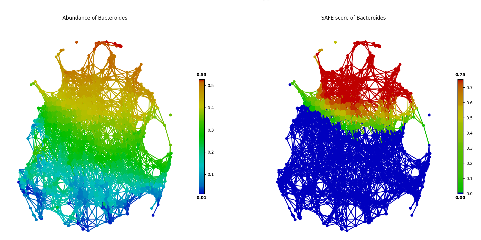
The following codes show how SAFE scores help to identify enriched nodes with significantly higher target values. In this case of FGFP microbiome study, a driver species (Bacteroides) enriched a group of connected nodes (the upper part of the network), which is more evident than a plotting with original species abundance values.
from scipy.spatial.distance import squareform, pdist
from sklearn.cluster import DBSCAN
from sklearn.preprocessing import MinMaxScaler

from tmap.netx.SAFE import SAFE_batch, get_SAFE_summary
from tmap.tda import mapper, Filter
from tmap.tda.cover import Cover
from tmap.tda.metric import Metric
from tmap.tda.plot import Color
from tmap.tda.utils import optimize_dbscan_eps
from tmap.test import load_data

# load taxa abundance data, sample metadata and precomputed distance matrix
X = load_data.FGFP_genus_profile()
metadata = load_data.FGFP_metadata_ready()
dm = squareform(pdist(X, metric='braycurtis'))

# TDA Step1. initiate a Mapper
tm = mapper.Mapper(verbose=1)

# TDA Step2. Projection
metric = Metric(metric="precomputed")
lens = [Filter.MDS(components=[0, 1], metric=metric,random_state=100)]
projected_X = tm.filter(dm, lens=lens)

# Step4. Covering, clustering & mapping
eps = optimize_dbscan_eps(X, threshold=95)
clusterer = DBSCAN(eps=eps, min_samples=3)
cover = Cover(projected_data=MinMaxScaler().fit_transform(projected_X), resolution=50, overlap=0.75)
graph = tm.map(data=X, cover=cover, clusterer=clusterer)
print(graph.info())
## Step 6. SAFE test for every features.
# target_feature = 'Faecalibacterium'
# target_feature = 'Prevotella'
target_feature = 'Bacteroides'
n_iter = 1000
enriched_scores = SAFE_batch(graph, metadata=X, n_iter=n_iter, _mode='enrich')
target_safe_score = enriched_scores.loc[:, target_feature]
## Step 7. Visualization
# colors by samples (target values in a list)
color = Color(target=X.loc[:, target_feature], dtype="numerical", target_by="sample")
graph.show(color=color,
           fig_size=(10, 10),
           node_size=15,
           notshow=False)

# colors by nodes (target values in a dictionary)
color = Color(target=target_safe_score, dtype="numerical", target_by="node")
graph.show(color=color,
           fig_size=(10, 10),
           node_size=15,
           notshow=False)
Of course, besides the visualization based on matplotlib, you could also use tm_plot or vis_progressX to visualize it.
from tmap.tda.plot import vis_progressX,tm_plot,Color
color = Color(target=target_safe_score, dtype='numerical', target_by="node")
tm_plot(graph,color=color,filename='SAFE_Bacteroides.html',auto_open=False)
Network-based Co-enrichment Analysis
Co-occurrence of microbial species can be used to infer relationship between species in a community. The concept of species co-occurrence is extended in tmap to a network-based co-enrichment analysis, which is a statistical analysis of species relationships based the TDA network structure.
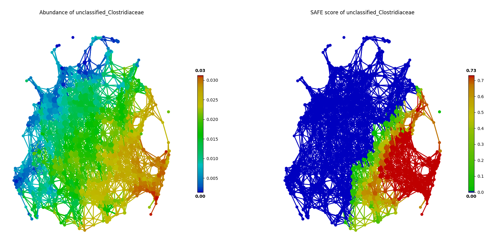
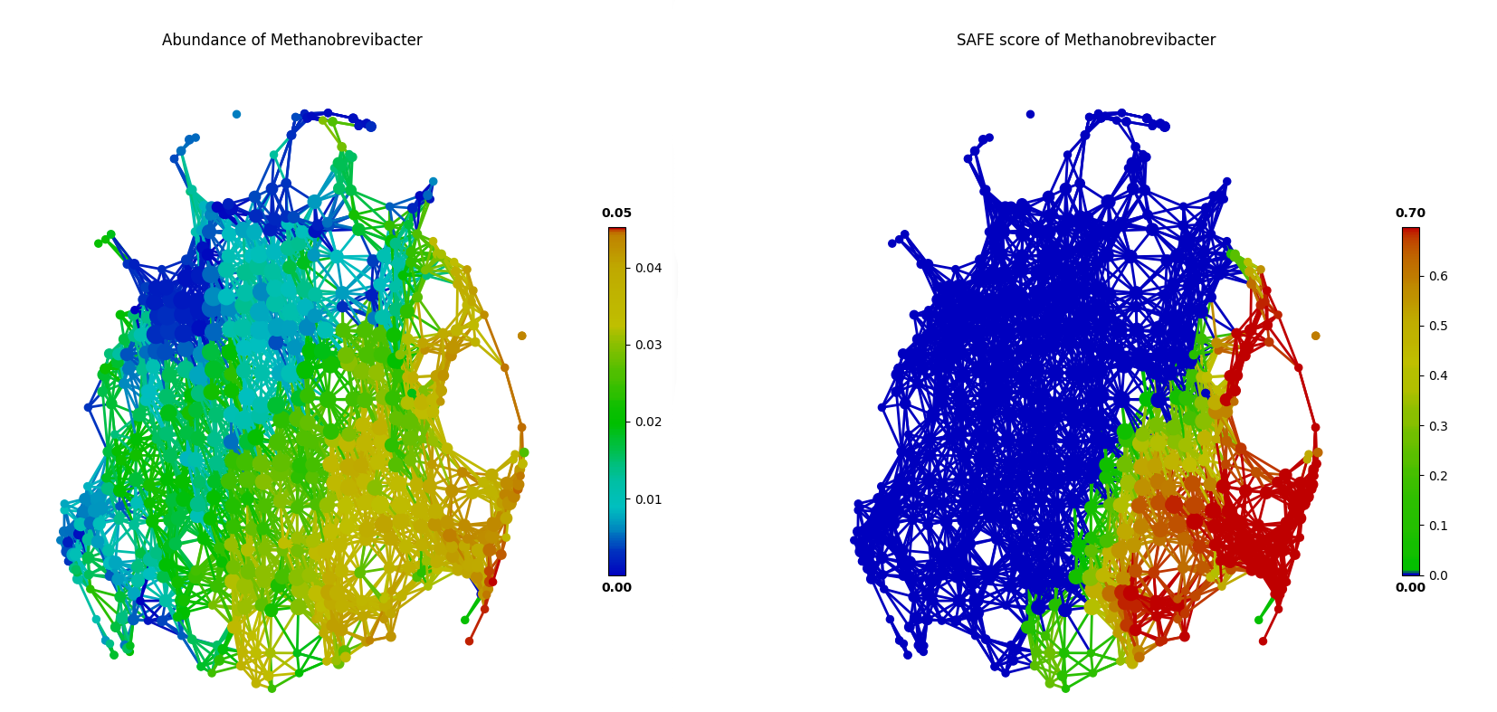
For example, using the FGFP microbiome dataset, we can test and visualize co-enrichment between identified driver species. As shown in the following figure, unclassified_Clostridiaceae and Methanobrevibacter are highly co-enriched in the network, which is more evident by SAFE scores than original species abundance.
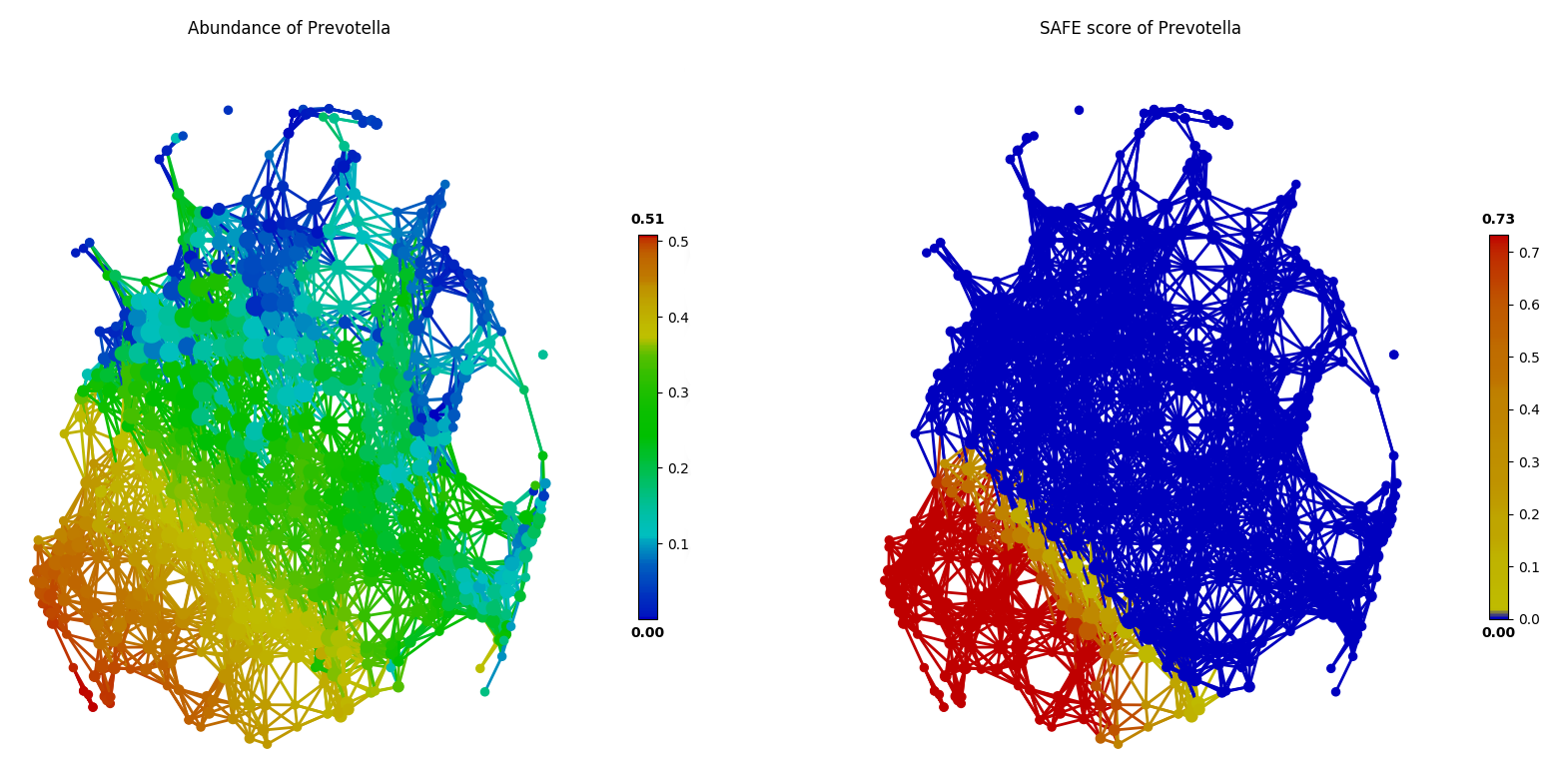
Mutually exclusive relationship between driver species can also be identified via this approach of network statistical analysis, based the SAFE scores rather than abundance. In the following figure, two known enterotype driver species, Prevotella and Bacteroides, are shown to have a mutually exclusive relationship in the FGFP microbiome dataset.
Network-based Association Analysis
tmap calculates SAFE scores for each node, given a target variable. We have implemented the SAFE_batch function in tmap for batch calculation for many target variables at the same time.
For target variables, they can be either species abundance or sample metadata. In this way, tmap provides two transformations on the input data. First, it transforms raw values to SAFE scores for a target variable. Meanwhile, it transforms samples into nodes, which are aggregations of a group of samples.
As below,
from tmap.netx.SAFE import SAFE_batch
n_iter = 1000
safe_scores = SAFE_batch(graph, metadata=X, n_iter=n_iter)
When we get the SAFE score which represented enrichment scale of specific feature, we could use a hard filter from assigned p-value to filter out a enriched region/nodes.
from tmap.netx.SAFE import get_significant_nodes
min_p_value = 1.0 / (n_iter + 1.0)
p_value = 0.05
SAFE_pvalue = np.log10(p_value) / np.log10(min_p_value)
enriched_centroides, enriched_nodes = get_significant_nodes(graph,safe_scores,SAFE_pvalue=SAFE_pvalue,r_neighbor=True)
Default, the function get_enriched_nodes only output the enriched nodes around the centroides. The difference between neighborhood and centroides could be find out at SAFE algorithm of ‘How tmap work’.
Upon the enriched area, we can perform a network-based co-enrichment relationship analysis for any pair of target variables. To do this, contingency tables with enriched/non-enriched and A/B features between each pairs of features was constructed. Fisher-exact test was performed based on each contingency table and corrected with by FDR (Benjamini/Hochberg).
from tmap.netx.coenrichment_analysis import pairwise_coenrichment
asso_pairs = pairwise_coenrichment(graph,safe_scores,n_iter=1000,p_value=0.05,_pre_cal_enriched=enriched_centroides)
# pre_cal_enriched could be none, and it will be calculated inside the pairwise_coenrichment function.